1. Introduction #
Excel is often used in connection with RPA, and typically most RPA software has built-in functionality to work with this. Therefore, this is more of a reference work, in addition there are links to read more about other things that can be used in connection with Excel.
| Name | Note | Link |
| Reference work | Everything about Excel, VBA functionality, useful examples, etc. | https://www.excel-easy.com/ |
| Course/Training | If you need an overview of the possibilities in Excel | https://www.w3schools.com/EXCEL/index.php |
| DAX | Used in both Power Pivot and Power BI | https://www.rpahelp.org/docs/dax-data-analysis-expressions/ |
| VBScript | VBScripting for Excel, where you can create a lot of functionality | VBScript – RPA Help |
| Power Pivot | Video walkthrough of Power Pivot | How to use Power Pivot in Excel | Full Tutorial |
| SQL to Excel files | It is possible to use SQL for Excel and CSV files, this is especially useful for larger sheets, and for RPA use | https://www.rpahelp.org/docs/sql/#1-toc-title |
1.1 365 – Turn off auto save #
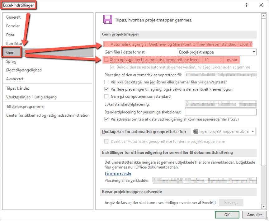
If you are using 365, it is an advantage to turn off auto-save, as this can interfere with the robot. One of the reasons is that it changes the window name when it saves.
2. Shortcut keys #
| Shortcut keys | Description |
| Search, copy, delete, mark | |
| Ctrl + Z | Undo |
| Ctrl + Y | Ready |
| Ctrl + C | Copy |
| Ctrl + X | Clip |
| Ctrl + V | Insert |
| Ctrl + B | Search |
| Ctrl + H | Search and replace |
| Ctrl + Shift + Down Arrow | Select selected column(s) down to the last used row |
| Ctrl + Shift + End | Select column down to last used row |
| Ctrl + A | Select the entire table of data |
| Ctrl + D | First copy the cell’s value down into the selected column |
| Sheet editing | |
| Ctrl + – | Delete row/column/cell |
| Ctrl + + | Insert row/column/cell |
| Shift + F11 | Insert new sheet |
| Ctrl + Page Up | Navigate forward to the next sheet |
| Ctrl + PgDn | Navigate back to previous sheets |
| Ribbon* | |
| Ctrl + F1 | Show or hide the ribbon |
| All | Enable shortcut keys on the ribbon |
| Files | |
| Ctrl + N | Open new folder/workbook |
| Ctrl + O | Open menu for opening files |
| Ctrl + S | Save |
| F12 | Save as |
| Ctrl + P | |
| Ctrl + F4 | Close open folder/workbook |
*Example when pressing All in a Danish version of Excel
3. Formatting cell values #
3.1 Numbers with leading 0 #
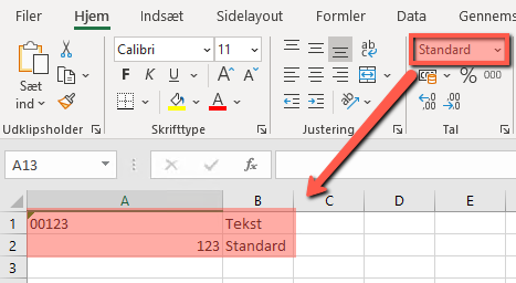
Convert the column / cell in question to text, otherwise this will automatically be translated to numbers, and remove the leading 0. See the Visual Basic Scripts for Excel section for a solution to this without printing.

3.2 Currency #
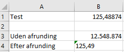
If currency or decimal numbers are to be inserted in Excel, they must be rounded up to 2 decimal places before doing this, otherwise Excel will translate it itself into a number without decimals, which can make the numbers extremely large.
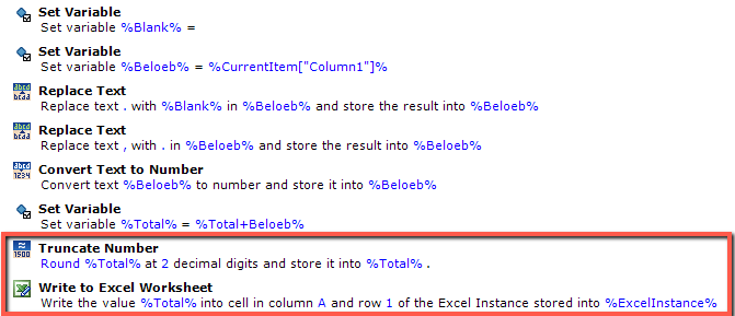
With the code above, Beloob starts as B1, and is then inserted directly into B3, and subsequently rounded and miscellaneous, and inserted into B4.
3.3 Dates #
Since Excel can occasionally translate dates to American format ( MM-dd-yyyy ) when pasted from the correct format, you can paste them as formulas instead. This bypasses Excel’s attempt to figure out the format itself.

4. Power Pivot #
Including a review of Power Pivot which is an alternative to Power BI. Cosmetic / layout related topics, such as how to make the report look like in the end, are not reviewed.
Attached is the completed sheet so you can continue playing yourself.
4.1 Retrieve data #
Before you can use Power Pivot , you must first use data in an Excel sheet. Then press Ctrl+T to convert this into a table that you can name. This will be our data base in the future. Please note that this will update itself if cells are added to the first free row at a later time.
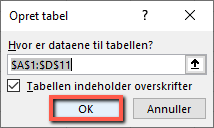
We now get a new menu, Table Design , and from here we can name our table something meaningful.

4.2 Pivot table #
To create tables etc., click Summarize with pivot table , and then OK .

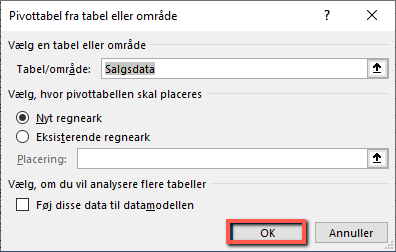
We can add an appropriate name for the new table at the top of the ribbon.

On the right we can choose which data we want to see, and this will be automatically updated in the table. You can also move it around, so you can choose which are columns, rows, values or filters.
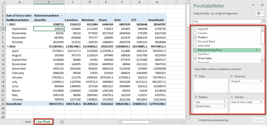
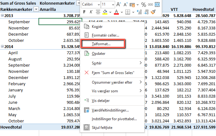
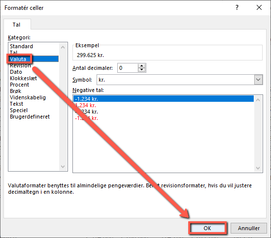
To change the Number Format, we can right-click and select Number Format… , and then switch to Currency .
4.3 Pivot chart #
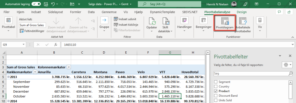
Charts can be inserted from the PivotTable Analysis menu, and then PivotChart .
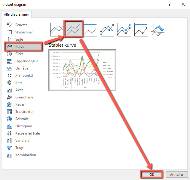
Under Curve, we choose a Stacked Curve to start with.
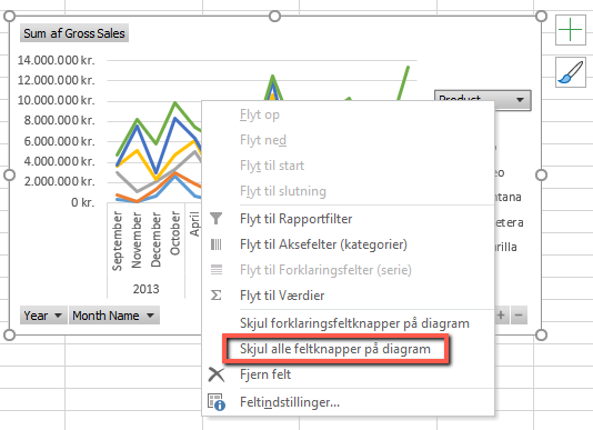
Field buttons can be used to further select what to display. In this case, we hide them away as they are not needed by right-clicking on the chart and selecting Hide all field buttons on chart .

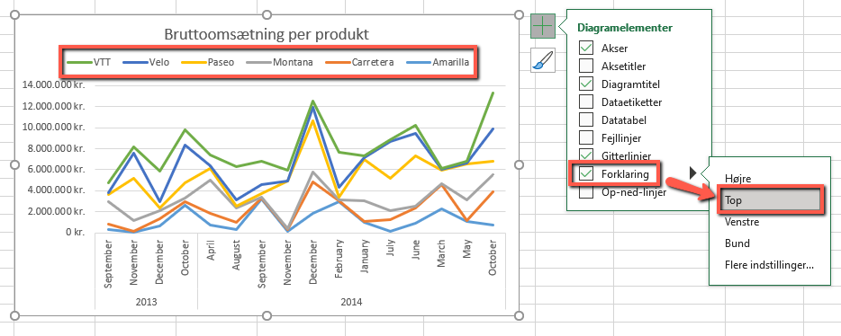
To insert a Chart Title, press + on the right and check this box.
We can move our Explanation , in this case product names, to the top at the same time.
4.4 Dashboard – Slicers / Sections (filters) #
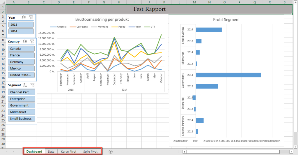
If you want a unified dashboard, it is easiest to cut / copy-paste the previous charts into a new sheet, where you can collect all the data. For this, we can create Slicers , which can be used to filter what is displayed. Select a chart, under PivotChart Analysis, press Insert Slicer , and select the desired filters.

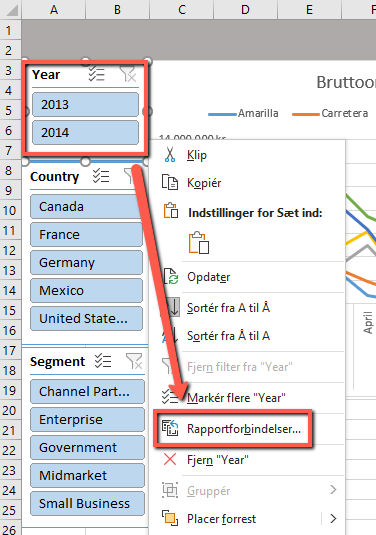
Currently, the previous slicers are only associated with our one chart. Right-click on these and select Report Connections… and check all the charts it should control. After that, the view will change to the selected charts when clicking on the different filters.

Alternatively, you can select a Slicer , and select Slicer Tool in the ribbon and then Report Connections .
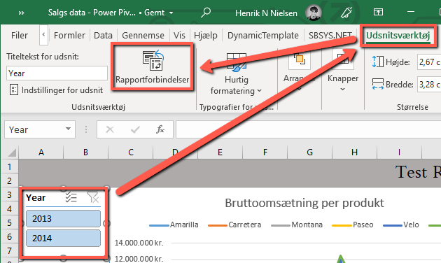
Then select the diagrams that are to be associated with the individual slicer .

It is easiest to create your dashboard as a separate sheet, data separately, and various pivots can be copy-pasted or cut into the dashboard as shown here.
